셀러 분류
def seller_group(row):
    if row['median'] >= 160:
        return 'high_price_seller'
    elif row['median'] >=90 :
        return 'medium_price_seller'
    else:
        return 'low_price_seller'
seller_price_stats['seller_type'] = seller_price_stats.apply(seller_group, axis=1)
seller_price_stats['seller_type'].value_counts(normalize=True)
color_map = {
'low_price_seller': 'blue',
'high_price_seller': 'red',
'medium_price_seller':'green'
}
plt.figure(figsize=(10,6))
for seller_type, color in color_map.items():
subset = seller_price_stats[seller_price_stats['seller_type'] == seller_type]
plt.scatter(subset['median'], subset['std'], label=seller_type, color=color, alpha=0.7)
plt.xlabel('Median Price')
plt.ylabel('Price Std')
plt.title('Seller Types Scatter Plot')
plt.legend()
plt.show()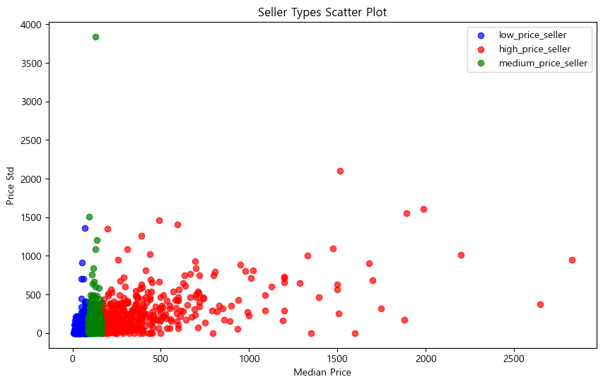
기존에는 고가 금액, 저가 금액, 다양한 금액 총 세 가지였는데, 애매한 금액을 포함하기 위해서 medium price를 추가했다.
# 1~2개, 3개 이상 그룹화
a = df.groupby('seller_id')['main_category'].nunique().reset_index()
a['category_group'] = a['main_category'].apply(lambda x: '1개' if x == 1 else '2개 이상')
# seller_type 정보 붙이기
# seller_type 정보 붙이기 (중복 제거 시 seller_id, seller_type만 남기도록)
seller_type = df[['seller_id', 'seller_type']].drop_duplicates()

a = a.merge(seller_type, on='seller_id', how='left')
plt.figure(figsize=(8, 6))
sns.countplot(
    x='category_group',
    hue='seller_type',
    data=a,
    palette='pastel'
)

plt.xlabel('판매 카테고리 수 그룹')
plt.ylabel('셀러 수')
plt.title('판매 카테고리 수 그룹별 셀러 수 (셀러타입별)')
plt.legend(title='셀러 타입')
plt.show()
대분류 카테고리는 총 11개정도 있지만, 보통 한 카테고리만 파는 판매자가 대부분이기 때문에 한 개와 두 개 이상으로 구분했다.
df_unique = df.drop_duplicates(subset=['seller_id', 'product_id'])
a = df_unique.groupby(['seller_type', 'main_category']).size().reset_index(name='count')

sns.barplot(x='seller_type', y='count', hue='main_category', data=a)
plt.legend(loc='upper left', bbox_to_anchor=(1, 1))
plt.show()
판매 금액대가 비슷해도, 카테고리를 여러개를 파냐 안파냐에 따라서 선호 카테고리가 달라진다.
# 셀러별로 고유 상품 기준 가격대 통계
seller_products = df.drop_duplicates(['seller_id', 'product_id'])[['seller_id', 'product_id', 'price']]
seller_price_stats = seller_products.groupby('seller_id')['price'].agg(['median','std']).reset_index()

# 가격대 그룹 (low/high)
def seller_group(row):
    if row['median'] >= 160:
        return 'high_price_seller'
    elif row['median'] >=90 :
        return 'medium_price_seller'
    else:
        return 'low_price_seller'

seller_price_stats['seller_type'] = seller_price_stats.apply(seller_group, axis=1)

# 카테고리 개수 및 그룹
category_counts = df.drop_duplicates(['seller_id', 'product_id', 'main_category']) \
    .groupby('seller_id')['main_category'].nunique().reset_index(name='category_count')

category_counts['category_group'] = category_counts['category_count'].apply(lambda x: '1개' if x == 1 else '2개 이상')

# seller_type + category_group
# 카테고리 그룹 merge
seller_price_stats = seller_price_stats.merge(category_counts[['seller_id', 'category_group']], on='seller_id', how='left')


# 4가지 조합 만들기
seller_price_stats['combined_group_4'] = seller_price_stats['seller_type'] + ' | ' + seller_price_stats['category_group']

# 4가지 조합 시각화
plt.figure(figsize=(10, 6))
sns.countplot(
    y='combined_group_4',
    data=seller_price_stats,
    palette='Set2',
    order=seller_price_stats['combined_group_4'].value_counts().index
)
plt.xlabel('셀러 수')
plt.ylabel('그룹 (가격대 | 카테고리 수)')
plt.title('6가지 조합 그룹별 셀러 수')
plt.show()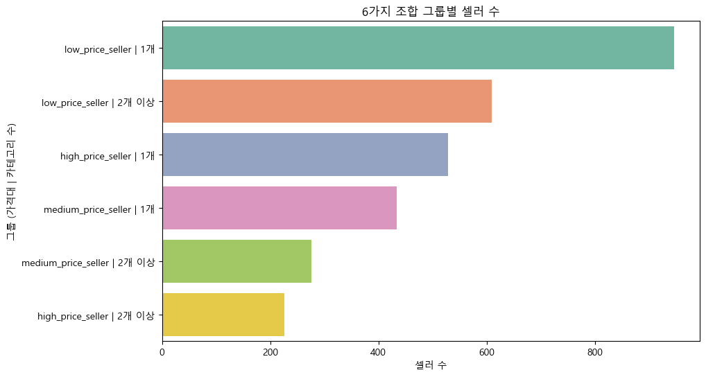
그래서 최종적으로 이렇게 총 6가지 분류가 나왔다.
'데이터분석 6기 > 본캠프' 카테고리의 다른 글
| 2025-06-10 배송기간 예측 모델 EDA (0) | 2025.06.10 |
|---|---|
| 2025-06-09 최종 프로젝트 비인기 카테고리 (0) | 2025.06.09 |
| 2025-06-05 spark 가상환경/virtual box, ubuntu, moba (1) | 2025.06.05 |
| 2025-06-04 최종 프로젝트 셀러 분석 (0) | 2025.06.04 |
| 2025-06-04 최종 프로젝트 데이터 전처리 (1) | 2025.06.04 |